How To Find Leading Term Of Polynomial

Type of mathematical expressions

For less simple aspects of the subject, run into Polynomial band.

The graph of a polynomial function of caste 3

In mathematics, a polynomial is an expression consisting of indeterminates (likewise called variables) and coefficients, that involves only the operations of addition, subtraction, multiplication, and non-negative integer exponentiation of variables. An example of a polynomial of a single indeterminate x is ten ⁱⁱ − 410 + 7. An example in three variables is ten ⁱⁱⁱ + twoxyz ² − yz + i.

Polynomials appear in many areas of mathematics and science. For example, they are used to course polynomial equations, which encode a wide range of problems, from simple word bug to complicated scientific problems; they are used to define polynomial functions, which appear in settings ranging from basic chemistry and physics to economics and social science; they are used in calculus and numerical analysis to approximate other functions. In advanced mathematics, polynomials are used to construct polynomial rings and algebraic varieties, which are central concepts in algebra and algebraic geometry.

Etymology [edit]

The discussion polynomial joins two diverse roots: the Greek poly, meaning "many", and the Latin nomen, or "name". Information technology was derived from the term binomial by replacing the Latin root bi- with the Greek poly-. That is, it means a sum of many terms (many monomials). The word polynomial was first used in the 17th century.^[ane]

Notation and terminology [edit]

The x occurring in a polynomial is commonly called a variable or an indeterminate. When the polynomial is considered as an expression, 10 is a fixed symbol which does not have whatsoever value (its value is "indeterminate"). However, when ane considers the role defined by the polynomial, then x represents the argument of the function, and is therefore called a "variable". Many authors utilize these two words interchangeably.

A polynomial P in the indeterminate x is commonly denoted either as P or as P(x). Formally, the name of the polynomial is P, not P(10), simply the use of the functional annotation P(x) dates from a time when the distinction between a polynomial and the associated function was unclear. Moreover, the functional notation is often useful for specifying, in a single phrase, a polynomial and its indeterminate. For example, "permit P(x) be a polynomial" is a shorthand for "let P exist a polynomial in the indeterminate 10". On the other paw, when it is not necessary to emphasize the name of the indeterminate, many formulas are much simpler and easier to read if the name(southward) of the indeterminate(due south) do not appear at each occurrence of the polynomial.

The ambiguity of having two notations for a single mathematical object may be formally resolved by considering the full general significant of the functional notation for polynomials. If a denotes a number, a variable, another polynomial, or, more generally, any expression, then P(a) denotes, by convention, the result of substituting a for ten in P. Thus, the polynomial P defines the function

${\displaystyle a\mapsto P(a),}$

which is the polynomial function associated to P. Ofttimes, when using this notation, one supposes that a is a number. However, i may use it over any domain where improver and multiplication are divers (that is, any band). In particular, if a is a polynomial and then P(a) is too a polynomial.

More specifically, when a is the indeterminate x, then the image of x by this role is the polynomial P itself (substituting x for x does not change annihilation). In other words,

${\displaystyle P(x)=P,}$

which justifies formally the existence of 2 notations for the aforementioned polynomial.

Definition [edit]

A polynomial expression is an expression that tin can be built from constants and symbols chosen variables or indeterminates by means of add-on, multiplication and exponentiation to a non-negative integer power. The constants are generally numbers, but may be any expression that exercise not involve the indeterminates, and represent mathematical objects that can be added and multiplied. 2 polynomial expressions are considered as defining the aforementioned polynomial if they may be transformed, one to the other, by applying the usual properties of commutativity, associativity and distributivity of add-on and multiplication. For example ${\displaystyle (ten-i)(x-2)}$ and ${\displaystyle x^{2}-3x+2}$ are two polynomial expressions that represent the same polynomial; and then, one writes ${\displaystyle (x-1)(x-two)=x^{2}-3x+2.}$

A polynomial in a single indeterminate x tin ever exist written (or rewritten) in the class

${\displaystyle a_{northward}x^{due north}+a_{n-i}x^{n-i}+\dotsb +a_{2}x^{ii}+a_{1}x+a_{0},}$

where ${\displaystyle a_{0},\ldots ,a_{north}}$ are constants that are called the coefficients of the polynomial, and ${\displaystyle x}$ is the indeterminate.^[2] The give-and-take "indeterminate" ways that ${\displaystyle x}$ represents no particular value, although any value may exist substituted for it. The mapping that assembly the issue of this substitution to the substituted value is a part, called a polynomial function.

This can be expressed more concisely by using summation notation:

${\displaystyle \sum _{one thousand=0}^{northward}a_{m}ten^{g}}$

That is, a polynomial tin can either exist zilch or can exist written as the sum of a finite number of non-nil terms. Each term consists of the product of a number – called the coefficient of the term^[a] – and a finite number of indeterminates, raised to nonnegative integer powers.

Classification [edit]

The exponent on an indeterminate in a term is called the degree of that indeterminate in that term; the degree of the term is the sum of the degrees of the indeterminates in that term, and the caste of a polynomial is the largest degree of any term with nonzero coefficient.^[three] Because x = x ¹ , the degree of an indeterminate without a written exponent is one.

A term with no indeterminates and a polynomial with no indeterminates are called, respectively, a constant term and a abiding polynomial.^[b] The degree of a abiding term and of a nonzero constant polynomial is 0. The caste of the cipher polynomial 0 (which has no terms at all) is mostly treated as not defined (but come across beneath).^[4]

For case:

${\displaystyle -5x^{two}y}$

is a term. The coefficient is −5, the indeterminates are ten and y , the degree of ten is ii, while the degree of y is one. The degree of the unabridged term is the sum of the degrees of each indeterminate in it, so in this example the caste is 2 + 1 = 3.

Forming a sum of several terms produces a polynomial. For case, the following is a polynomial:

${\displaystyle \underbrace {_{\,}3x^{2}} _{\begin{smallmatrix}\mathrm {term} \\\mathrm {1} \stop{smallmatrix}}\underbrace {-_{\,}5x} _{\begin{smallmatrix}\mathrm {term} \\\mathrm {2} \end{smallmatrix}}\underbrace {+_{\,}4} _{\begin{smallmatrix}\mathrm {term} \\\mathrm {3} \end{smallmatrix}}.}$

Information technology consists of three terms: the first is caste ii, the second is caste one, and the third is degree zero.

Polynomials of small degree have been given specific names. A polynomial of degree nix is a abiding polynomial, or simply a constant. Polynomials of caste i, 2 or three are respectively linear polynomials, quadratic polynomials and cubic polynomials.^[3] For college degrees, the specific names are non usually used, although quartic polynomial (for degree 4) and quintic polynomial (for caste five) are sometimes used. The names for the degrees may be practical to the polynomial or to its terms. For case, the term 2x in x ² + 2x + i is a linear term in a quadratic polynomial.

The polynomial 0, which may be considered to accept no terms at all, is called the zero polynomial. Unlike other constant polynomials, its degree is non zip. Rather, the degree of the naught polynomial is either left explicitly undefined, or divers every bit negative (either −ane or −∞).^[5] The zero polynomial is likewise unique in that it is the but polynomial in one indeterminate that has an infinite number of roots. The graph of the nix polynomial, f(x) = 0, is the x-axis.

In the case of polynomials in more than i indeterminate, a polynomial is called homogeneous of caste n if all of its not-nil terms take degree n . The naught polynomial is homogeneous, and, equally a homogeneous polynomial, its degree is undefined.^[c] For instance, x ⁱⁱⁱ y ² + 710 ² y ⁱⁱⁱ − 3x ⁵ is homogeneous of caste 5. For more details, see Homogeneous polynomial.

The commutative law of addition tin be used to rearrange terms into any preferred gild. In polynomials with ane indeterminate, the terms are normally ordered according to degree, either in "descending powers of ten ", with the term of largest degree first, or in "ascending powers of x ". The polynomial iiix ² - v10 + 4 is written in descending powers of x . The first term has coefficient 3, indeterminate ten , and exponent 2. In the 2d term, the coefficient is −v . The third term is a constant. Because the caste of a non-zero polynomial is the largest degree of any 1 term, this polynomial has degree ii.^[6]

Two terms with the same indeterminates raised to the same powers are called "similar terms" or "like terms", and they can be combined, using the distributive law, into a single term whose coefficient is the sum of the coefficients of the terms that were combined. It may happen that this makes the coefficient 0.^[seven] Polynomials can exist classified past the number of terms with nonzero coefficients, then that a one-term polynomial is called a monomial,^[d] a two-term polynomial is called a binomial, and a three-term polynomial is called a trinomial. The term "quadrinomial" is occasionally used for a four-term polynomial.

A real polynomial is a polynomial with existent coefficients. When it is used to define a function, the domain is not so restricted. However, a real polynomial function is a office from the reals to the reals that is defined past a real polynomial. Similarly, an integer polynomial is a polynomial with integer coefficients, and a complex polynomial is a polynomial with complex coefficients.

A polynomial in i indeterminate is called a univariate polynomial, a polynomial in more than ane indeterminate is called a multivariate polynomial. A polynomial with 2 indeterminates is called a bivariate polynomial.^[ii] These notions refer more to the kind of polynomials one is generally working with than to private polynomials; for case, when working with univariate polynomials, i does not exclude constant polynomials (which may event from the subtraction of not-constant polynomials), although strictly speaking, constant polynomials practise not contain any indeterminates at all. It is possible to further classify multivariate polynomials as bivariate, trivariate, and so on, according to the maximum number of indeterminates allowed. Again, so that the fix of objects under consideration be closed under subtraction, a study of trivariate polynomials unremarkably allows bivariate polynomials, and so on. It is also common to say simply "polynomials in x, y , and z ", listing the indeterminates allowed.

The evaluation of a polynomial consists of substituting a numerical value to each indeterminate and conveying out the indicated multiplications and additions. For polynomials in one indeterminate, the evaluation is unremarkably more efficient (lower number of arithmetics operations to perform) using Horner's method:

${\displaystyle (((((a_{n}x+a_{n-1})x+a_{northward-2})x+\dotsb +a_{3})x+a_{2})x+a_{1})10+a_{0}.}$

Arithmetics [edit]

Addition and subtraction [edit]

Polynomials can be added using the associative law of add-on (grouping all their terms together into a single sum), possibly followed past reordering (using the commutative law) and combining of like terms.^{[7] [eight]} For example, if

${\displaystyle P=3x^{2}-2x+5xy-2}$ and ${\displaystyle Q=-3x^{two}+3x+4y^{ii}+8}$

then the sum

${\displaystyle P+Q=3x^{2}-2x+5xy-2-3x^{2}+3x+4y^{2}+8}$

can be reordered and regrouped every bit

${\displaystyle P+Q=(3x^{2}-3x^{2})+(-2x+3x)+5xy+4y^{2}+(8-2)}$

then simplified to

${\displaystyle P+Q=x+5xy+4y^{2}+vi.}$

When polynomials are added together, the effect is some other polynomial.^[9]

Subtraction of polynomials is similar.

Multiplication [edit]

Polynomials can likewise exist multiplied. To expand the product of ii polynomials into a sum of terms, the distributive law is repeatedly applied, which results in each term of one polynomial being multiplied past every term of the other.^[7] For example, if

${\displaystyle {\begin{aligned}\colour {Red}P&\color {Red}{=2x+3y+five}\\\colour {Blue}Q&\color {Blue}{=2x+5y+xy+1}\terminate{aligned}}}$

and then

${\displaystyle {\brainstorm{assortment}{rccrcrcrcr}{\color {Blood-red}{P}}{\color {Blue}{Q}}&{=}&&({\color {Red}{2x}}\cdot {\colour {Blueish}{2x}})&+&({\color {Ruddy}{2x}}\cdot {\colour {Blueish}{5y}})&+&({\colour {Reddish}{2x}}\cdot {\color {Blue}{xy}})&+&({\color {Red}{2x}}\cdot {\color {Blue}{1}})\\&&+&({\colour {Red}{3y}}\cdot {\colour {Blue}{2x}})&+&({\color {Red}{3y}}\cdot {\color {Blueish}{5y}})&+&({\color {Cerise}{3y}}\cdot {\colour {Blue}{xy}})&+&({\color {Red}{3y}}\cdot {\color {Blue}{1}})\\&&+&({\color {Crimson}{5}}\cdot {\color {Blueish}{2x}})&+&({\color {Cherry-red}{v}}\cdot {\color {Blue}{5y}})&+&({\colour {Red}{5}}\cdot {\colour {Blue}{xy}})&+&({\colour {Carmine}{5}}\cdot {\colour {Blueish}{i}})\end{assortment}}}$

Carrying out the multiplication in each term produces

${\displaystyle {\begin{assortment}{rccrcrcrcr}PQ&=&&4x^{2}&+&10xy&+&2x^{ii}y&+&2x\\&&+&6xy&+&15y^{2}&+&3xy^{ii}&+&3y\\&&+&10x&+&25y&+&5xy&+&five.\end{array}}}$

Combining like terms yields

${\displaystyle {\begin{array}{rcccrcrcrcr}PQ&=&&4x^{two}&+&(10xy+6xy+5xy)&+&2x^{2}y&+&(2x+10x)\\&&+&15y^{2}&+&3xy^{2}&+&(3y+25y)&+&v\end{array}}}$

which can be simplified to

${\displaystyle PQ=4x^{2}+21xy+2x^{ii}y+12x+15y^{ii}+3xy^{ii}+28y+five.}$

As in the example, the product of polynomials is always a polynomial.^{[ix] [four]}

Limerick [edit]

Given a polynomial ${\displaystyle f}$ of a single variable and some other polynomial thou of any number of variables, the limerick ${\displaystyle f\circ g}$ is obtained by substituting each copy of the variable of the first polynomial by the second polynomial.^[iv] For example, if ${\displaystyle f(x)=10^{two}+2x}$ and ${\displaystyle g(10)=3x+two}$ then

$${\displaystyle (f\circ grand)(x)=f(thou(x))=(3x+2)^{2}+two(3x+2).}$$

A composition may be expanded to a sum of terms using the rules for multiplication and division of polynomials. The composition of two polynomials is another polynomial.^[x]

Segmentation [edit]

The division of 1 polynomial by another is not typically a polynomial. Instead, such ratios are a more general family of objects, called rational fractions, rational expressions, or rational functions, depending on context.^[xi] This is coordinating to the fact that the ratio of two integers is a rational number, not necessarily an integer.^{[12] [thirteen]} For case, the fraction 1/(x ⁱⁱ + 1) is non a polynomial, and it cannot be written as a finite sum of powers of the variable 10.

For polynomials in one variable, at that place is a notion of Euclidean partition of polynomials, generalizing the Euclidean division of integers.^[e] This notion of the sectionalization a(x)/b(x) results in two polynomials, a quotient q(x) and a remainder r(10), such that a = b q + r and degree(r) < caste(b). The caliber and residuum may be computed by whatsoever of several algorithms, including polynomial long division and constructed division.^[14]

When the denominator b(x) is monic and linear, that is, b(x) = x − c for some constant c, then the polynomial rest theorem asserts that the balance of the sectionalisation of a(x) by b(ten) is the evaluation a(c).^[thirteen] In this instance, the caliber may be computed by Ruffini'south rule, a special case of constructed division.^[15]

Factoring [edit]

All polynomials with coefficients in a unique factorization domain (for example, the integers or a field) also have a factored form in which the polynomial is written as a product of irreducible polynomials and a constant. This factored form is unique upwards to the guild of the factors and their multiplication by an invertible constant. In the case of the field of complex numbers, the irreducible factors are linear. Over the real numbers, they have the degree either one or 2. Over the integers and the rational numbers the irreducible factors may have any degree.^[16] For instance, the factored form of

${\displaystyle 5x^{three}-5}$

is

${\displaystyle 5(x-1)\left(10^{2}+x+one\right)}$

over the integers and the reals, and

${\displaystyle 5(x-one)\left(ten+{\frac {1+i{\sqrt {three}}}{2}}\correct)\left(x+{\frac {1-i{\sqrt {3}}}{2}}\right)}$

over the complex numbers.

The computation of the factored form, called factorization is, in general, too hard to exist done past hand-written ciphering. However, efficient polynomial factorization algorithms are bachelor in virtually computer algebra systems.

Calculus [edit]

Calculating derivatives and integrals of polynomials is particularly simple, compared to other kinds of functions. The derivative of the polynomial

$${\displaystyle P=a_{n}x^{n}+a_{n-i}x^{north-one}+\dots +a_{2}x^{2}+a_{one}10+a_{0}=\sum _{i=0}^{north}a_{i}x^{i}}$$

with respect to x is the polynomial

$${\displaystyle na_{n}ten^{north-1}+(due north-1)a_{north-i}10^{n-2}+\dots +2a_{two}x+a_{1}=\sum _{i=1}^{due north}ia_{i}x^{i-1}.}$$

Similarly, the general antiderivative (or indefinite integral) of ${\displaystyle P}$ is

$${\displaystyle {\frac {a_{northward}ten^{northward+one}}{n+1}}+{\frac {a_{n-ane}x^{northward}}{n}}+\dots +{\frac {a_{2}ten^{3}}{3}}+{\frac {a_{i}x^{2}}{2}}+a_{0}10+c=c+\sum _{i=0}^{north}{\frac {a_{i}ten^{i+ane}}{i+1}}}$$

where c is an arbitrary constant. For case, antiderivatives of x ² + one have the form 1 / 3 x ³ + ten + c .

For polynomials whose coefficients come from more abstract settings (for example, if the coefficients are integers modulo some prime number p , or elements of an arbitrary band), the formula for the derivative can still exist interpreted formally, with the coefficient ka _k understood to mean the sum of yard copies of a _yard . For example, over the integers modulo p , the derivative of the polynomial ten ^p + x is the polynomial 1.^[17]

Polynomial functions [edit]

A polynomial part is a role that can be defined by evaluating a polynomial. More than precisely, a function f of ane argument from a given domain is a polynomial function if at that place exists a polynomial

${\displaystyle a_{n}ten^{north}+a_{n-1}10^{n-one}+\cdots +a_{2}x^{2}+a_{1}x+a_{0}}$

that evaluates to ${\displaystyle f(x)}$ for all ten in the domain of f (here, n is a not-negative integer and a ₀, a ₁, a _two, ..., a_n are constant coefficients). Generally, unless otherwise specified, polynomial functions have complex coefficients, arguments, and values. In item, a polynomial, restricted to accept existent coefficients, defines a function from the complex numbers to the circuitous numbers. If the domain of this function is also restricted to the reals, the resulting part is a real function that maps reals to reals.

For example, the part f , defined by

${\displaystyle f(x)=10^{3}-x,}$

is a polynomial function of one variable. Polynomial functions of several variables are similarly defined, using polynomials in more than one indeterminate, as in

${\displaystyle f(x,y)=2x^{iii}+4x^{ii}y+xy^{5}+y^{2}-7.}$

According to the definition of polynomial functions, there may be expressions that obviously are not polynomials but nevertheless define polynomial functions. An example is the expression ${\displaystyle \left({\sqrt {1-x^{2}}}\correct)^{2},}$ which takes the same values as the polynomial ${\displaystyle 1-10^{2}}$ on the interval ${\displaystyle [-ane,1]}$ , and thus both expressions define the same polynomial function on this interval.

Every polynomial part is continuous, smooth, and entire.

Graphs [edit]

• 

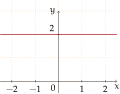
  Polynomial of degree 0:
  f(10) = two

• 

  Polynomial of degree ane:
  f(ten) = iix + 1

• 

  Polynomial of degree 2:
  f(10) = x ⁱⁱ − x − 2
  = (x + 1)(x − 2)

• 

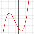
  Polynomial of degree 3:
  f(ten) = x ^three/4 + threex ²/4 − iiix/two − 2
  = 1/4 (x + four)(x + one)(x − 2)

• 

  Polynomial of degree 4:
  f(10) = ane/14 (10 + four)(x + ane)(x − 1)(10 − 3)
  + 0.5

• 

  Polynomial of caste 5:
  f(x) = 1/20 (10 + 4)(x + 2)(10 + one)(ten − 1)
  (x − iii) + 2

• 

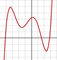
  Polynomial of degree half-dozen:
  f(x) = ane/100 (10 ^{half dozen} − 2ten ⁵ − 26x ^four + 28x ³
  + 145ten ² − 26ten − lxxx)

• 

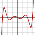
  Polynomial of degree 7:
  f(x) = (x − 3)(10 − 2)(ten − i)(x)(x + 1)(x + 2)
  (x + three)

A polynomial role in one existent variable can be represented past a graph.

• The graph of the zero polynomial

  f(ten) = 0

  is the 10 -centrality.
• The graph of a degree 0 polynomial

  f(x) = a ₀ , where a ₀ ≠ 0,

  is a horizontal line with y -intercept a ₀
• The graph of a degree 1 polynomial (or linear function)

  f(x) = a ₀ + a ₁ x , where a _one ≠ 0,

  is an oblique line with y -intercept a ₀ and slope a ₁ .
• The graph of a degree 2 polynomial

  f(x) = a ₀ + a ₁ x + a _two x ^two , where a ₂ ≠ 0

  is a parabola.
• The graph of a degree 3 polynomial

  f(x) = a ₀ + a ₁ 10 + a _two x ^two + a ₃ x ³ , where a ₃ ≠ 0

  is a cubic curve.
• The graph of any polynomial with degree 2 or greater

  f(x) = a ₀ + a ₁ x + a ₂ x ² + ⋯ + a _north ten ^{due north} , where a _{due north} ≠ 0 and n ≥ two

  is a continuous non-linear curve.

A non-abiding polynomial function tends to infinity when the variable increases indefinitely (in absolute value). If the degree is higher than one, the graph does not take any asymptote. Information technology has two parabolic branches with vertical direction (ane co-operative for positive x and i for negative ten).

Polynomial graphs are analyzed in calculus using intercepts, slopes, concavity, and finish behavior.

Equations [edit]

A polynomial equation, besides called an algebraic equation, is an equation of the form^[18]

${\displaystyle a_{n}ten^{n}+a_{northward-i}10^{north-1}+\dotsb +a_{2}ten^{2}+a_{ane}x+a_{0}=0.}$

For example,

${\displaystyle 3x^{2}+4x-5=0}$

is a polynomial equation.

When considering equations, the indeterminates (variables) of polynomials are also called unknowns, and the solutions are the possible values of the unknowns for which the equality is true (in general more than than one solution may exist). A polynomial equation stands in dissimilarity to a polynomial identity like (10 + y)(ten − y) = x ² − y ^two , where both expressions stand for the aforementioned polynomial in unlike forms, and as a consequence whatever evaluation of both members gives a valid equality.

In unproblematic algebra, methods such as the quadratic formula are taught for solving all first degree and second degree polynomial equations in one variable. In that location are also formulas for the cubic and quartic equations. For higher degrees, the Abel–Ruffini theorem asserts that there can not exist a full general formula in radicals. However, root-finding algorithms may be used to find numerical approximations of the roots of a polynomial expression of whatever degree.

The number of solutions of a polynomial equation with existent coefficients may not exceed the caste, and equals the degree when the complex solutions are counted with their multiplicity. This fact is called the key theorem of algebra.

Solving equations [edit]

A root of a nonzero univariate polynomial P is a value a of x such that P(a) = 0. In other words, a root of P is a solutions of the polynomial equation P(x) = 0 or a zero of the polynomial function defined by P . In the case of the zero polynomial, every number is ia zero of the corresponding function, and the concept of root is rarely cosidered.

A number a is a root of a polynomial P if and merely if the linear polynomial x − a divides P , that is if there is another polynomial Q such that P = (x − a) Q. It may happen that a ability (greater than 1) of x − a divides P ; in this case, a is a multiple root of P , and otherwise a is simple root of P . If P is a nonzero polynomial, there is a highest power m such that (x − a) ^m divides P , which is called the multiplicity of a as a root of P . The number of roots of a nonzero polynomial P , counted with their respective multiplicities, cannot exceed the degree of P ,^[19] and equals this caste if all circuitous roots are considered (this is a outcome of the fundamental theorem of algebra. The coefficients of a polynomial and its roots are related by Vieta's formulas.

Some polynomials, such as ten ² + one, exercise not take any roots among the real numbers. If, however, the set of accustomed solutions is expanded to the complex numbers, every non-constant polynomial has at least one root; this is the fundamental theorem of algebra. By successively dividing out factors ten − a , ane sees that any polynomial with complex coefficients tin exist written as a constant (its leading coefficient) times a product of such polynomial factors of degree ane; as a consequence, the number of (complex) roots counted with their multiplicities is exactly equal to the caste of the polynomial.

In that location may be several meanings of "solving an equation". One may want to limited the solutions as explicit numbers; for example, the unique solution of twox − ane = 0 is 1/2. Unfortunately, this is, in full general, impossible for equations of degree greater than one, and, since the ancient times, mathematicians have searched to express the solutions as algebraic expression; for case the golden ratio ${\displaystyle (ane+{\sqrt {5}})/2}$ is the unique positive solution of ${\displaystyle x^{2}-x-1=0.}$ In the aboriginal times, they succeeded only for degrees one and two. For quadratic equations, the quadratic formula provides such expressions of the solutions. Since the 16th century, similar formulas (using cube roots in addition to square roots), only much more complicated are known for equations of degree three and four (encounter cubic equation and quartic equation). But formulas for degree v and higher eluded researchers for several centuries. In 1824, Niels Henrik Abel proved the hitting event that there are equations of caste 5 whose solutions cannot be expressed by a (finite) formula, involving only arithmetic operations and radicals (come across Abel–Ruffini theorem). In 1830, Évariste Galois proved that almost equations of caste college than 4 cannot be solved by radicals, and showed that for each equation, 1 may decide whether it is solvable past radicals, and, if it is, solve it. This result marked the start of Galois theory and group theory, 2 important branches of mod algebra. Galois himself noted that the computations implied past his method were impracticable. Nevertheless, formulas for solvable equations of degrees 5 and 6 have been published (see quintic function and sextic equation).

When there is no algebraic expression for the roots, and when such an algebraic expression exists but is as well complicated to exist useful, the unique way of solving is to compute numerical approximations of the solutions.^[20] There are many methods for that; some are restricted to polynomials and others may apply to whatever continuous function. The about efficient algorithms allow solving hands (on a computer) polynomial equations of degree higher than 1,000 (see Root-finding algorithm).

For polynomials in more than one indeterminate, the combinations of values for the variables for which the polynomial function takes the value zero are by and large called zeros instead of "roots". The study of the sets of zeros of polynomials is the object of algebraic geometry. For a set of polynomial equations in several unknowns, there are algorithms to decide whether they have a finite number of circuitous solutions, and, if this number is finite, for computing the solutions. See Organisation of polynomial equations.

The special case where all the polynomials are of degree one is chosen a system of linear equations, for which some other range of different solution methods be, including the classical Gaussian elimination.

A polynomial equation for which ane is interested only in the solutions which are integers is called a Diophantine equation. Solving Diophantine equations is generally a very hard task. It has been proved that there cannot be any general algorithm for solving them, and even for deciding whether the prepare of solutions is empty (meet Hilbert'due south tenth trouble). Some of the most famous problems that accept been solved during the fifty final years are related to Diophantine equations, such equally Fermat'due south Concluding Theorem.

Generalizations [edit]

At that place are several generalizations of the concept of polynomials.

Trigonometric polynomials [edit]

A trigonometric polynomial is a finite linear combination of functions sin(nx) and cos(nx) with north taking on the values of one or more natural numbers.^[21] The coefficients may be taken equally real numbers, for existent-valued functions.

If sin(nx) and cos(nx) are expanded in terms of sin(x) and cos(ten), a trigonometric polynomial becomes a polynomial in the ii variables sin(ten) and cos(ten) (using List of trigonometric identities#Multiple-bending formulae). Conversely, every polynomial in sin(x) and cos(ten) may be converted, with Product-to-sum identities, into a linear combination of functions sin(nx) and cos(nx). This equivalence explains why linear combinations are called polynomials.

For complex coefficients, at that place is no departure betwixt such a function and a finite Fourier series.

Trigonometric polynomials are widely used, for example in trigonometric interpolation practical to the interpolation of periodic functions. They are used also in the detached Fourier transform.

Matrix polynomials [edit]

A matrix polynomial is a polynomial with square matrices equally variables.^[22] Given an ordinary, scalar-valued polynomial

${\displaystyle P(x)=\sum _{i=0}^{due north}{a_{i}x^{i}}=a_{0}+a_{1}x+a_{2}x^{2}+\cdots +a_{n}x^{n},}$

this polynomial evaluated at a matrix A is

${\displaystyle P(A)=\sum _{i=0}^{northward}{a_{i}A^{i}}=a_{0}I+a_{1}A+a_{2}A^{ii}+\cdots +a_{due north}A^{n},}$

where I is the identity matrix.^[23]

A matrix polynomial equation is an equality between two matrix polynomials, which holds for the specific matrices in question. A matrix polynomial identity is a matrix polynomial equation which holds for all matrices A in a specified matrix ring G_n (R).

Laurent polynomials [edit]

Laurent polynomials are like polynomials, but let negative powers of the variable(due south) to occur.

Rational functions [edit]

A rational fraction is the quotient (algebraic fraction) of two polynomials. Any algebraic expression that tin can be rewritten as a rational fraction is a rational office.

While polynomial functions are divers for all values of the variables, a rational office is defined but for the values of the variables for which the denominator is not aught.

The rational fractions include the Laurent polynomials, but do not limit denominators to powers of an indeterminate.

Power series [edit]

Formal power series are similar polynomials, but permit infinitely many non-nothing terms to occur, so that they do not have finite degree. Unlike polynomials they cannot in full general exist explicitly and fully written down (merely like irrational numbers cannot), but the rules for manipulating their terms are the same every bit for polynomials. Non-formal ability series likewise generalize polynomials, simply the multiplication of two power series may not converge.

Other examples [edit]

A bivariate polynomial where the 2d variable is substituted past an exponential function applied to the beginning variable, for example P(10, e ¹⁰ ), may exist called an exponential polynomial.

Polynomial band [edit]

A polynomial f over a commutative band R is a polynomial all of whose coefficients belong to R . It is straightforward to verify that the polynomials in a given fix of indeterminates over R form a commutative ring, chosen the polynomial ring in these indeterminates, denoted ${\displaystyle R[x]}$ in the univariate case and ${\displaystyle R[x_{1},\ldots ,x_{n}]}$ in the multivariate case.

One has

${\displaystyle R[x_{1},\ldots ,x_{north}]=\left(R[x_{one},\ldots ,x_{n-1}]\right)[x_{due north}].}$

So, most of the theory of the multivariate case can be reduced to an iterated univariate case.

The map from R to R[ten] sending r to itself considered equally a abiding polynomial is an injective ring homomorphism, by which R is viewed as a subring of R[ten]. In particular, R[x] is an algebra over R .

One can retrieve of the ring R[x] as arising from R by adding one new element 10 to R, and extending in a minimal style to a ring in which x satisfies no other relations than the obligatory ones, plus commutation with all elements of R (that is xr = rx ). To do this, one must add all powers of x and their linear combinations equally well.

Formation of the polynomial band, together with forming gene rings by factoring out ideals, are important tools for amalgam new rings out of known ones. For instance, the ring (in fact field) of complex numbers, which tin be constructed from the polynomial ring R[x] over the real numbers by factoring out the platonic of multiples of the polynomial x ² + 1. Another instance is the construction of finite fields, which proceeds similarly, starting out with the field of integers modulo some prime number as the coefficient band R (come across modular arithmetic).

If R is commutative, so one can associate with every polynomial P in R[x] a polynomial function f with domain and range equal to R . (More generally, i can have domain and range to be any same unital associative algebra over R .) One obtains the value f(r) by substitution of the value r for the symbol x in P . Ane reason to distinguish betwixt polynomials and polynomial functions is that, over some rings, different polynomials may give rising to the same polynomial office (see Fermat's trivial theorem for an example where R is the integers modulo p ). This is not the case when R is the real or complex numbers, whence the two concepts are not always distinguished in analysis. An fifty-fifty more than of import reason to distinguish between polynomials and polynomial functions is that many operations on polynomials (like Euclidean division) require looking at what a polynomial is composed of equally an expression rather than evaluating it at some abiding value for x .

Divisibility [edit]

If R is an integral domain and f and g are polynomials in R[x], it is said that f divides yard or f is a divisor of yard if there exists a polynomial q in R[x] such that f q = g . If ${\displaystyle a\in R,}$ then a is a root of f if and only ${\displaystyle x-a}$ divides f. In this case, the caliber tin can be computed using the polynomial long division.^{[24] [25]}

If F is a field and f and g are polynomials in F[x] with g ≠ 0, then there exist unique polynomials q and r in F[ten] with

${\displaystyle f=q\,k+r}$

and such that the caste of r is smaller than the degree of grand (using the convention that the polynomial 0 has a negative degree). The polynomials q and r are uniquely adamant by f and g . This is called Euclidean division, division with balance or polynomial long sectionalization and shows that the band F[x] is a Euclidean domain.

Analogously, prime number polynomials (more than correctly, irreducible polynomials) can be defined as non-zip polynomials which cannot be factorized into the product of two non-abiding polynomials. In the case of coefficients in a ring, "non-constant" must be replaced by "non-constant or non-unit" (both definitions concord in the case of coefficients in a field). Any polynomial may be decomposed into the product of an invertible constant by a product of irreducible polynomials. If the coefficients belong to a field or a unique factorization domain this decomposition is unique upwardly to the society of the factors and the multiplication of any non-unit factor by a unit (and sectionalisation of the unit of measurement cistron by the same unit). When the coefficients belong to integers, rational numbers or a finite field, at that place are algorithms to test irreducibility and to compute the factorization into irreducible polynomials (see Factorization of polynomials). These algorithms are not practicable for hand-written ciphering, but are bachelor in whatever computer algebra organization. Eisenstein's criterion tin also exist used in some cases to determine irreducibility.

Applications [edit]

Positional notation [edit]

In modern positional numbers systems, such as the decimal system, the digits and their positions in the representation of an integer, for example, 45, are a shorthand notation for a polynomial in the radix or base, in this case, 4 × x^ane + 5 × ten⁰ . Equally some other example, in radix v, a string of digits such equally 132 denotes the (decimal) number ane × 5² + 3 × 5ⁱ + 2 × v⁰ = 42. This representation is unique. Allow b be a positive integer greater than 1. Then every positive integer a can exist expressed uniquely in the form

${\displaystyle a=r_{m}b^{k}+r_{thousand-1}b^{m-one}+\dotsb +r_{1}b+r_{0},}$

where m is a nonnegative integer and the r's are integers such that

0 < r _m < b and 0 ≤ r _i < b for i = 0, one, . . . , m − 1.^[26]

Interpolation and approximation [edit]

The uncomplicated construction of polynomial functions makes them quite useful in analyzing general functions using polynomial approximations. An important instance in calculus is Taylor'due south theorem, which roughly states that every differentiable function locally looks similar a polynomial function, and the Stone–Weierstrass theorem, which states that every continuous function defined on a compact interval of the real centrality tin can be approximated on the whole interval as closely as desired by a polynomial function. Practical methods of approximation include polynomial interpolation and the use of splines.^[27]

Other applications [edit]

Polynomials are ofttimes used to encode information most some other object. The feature polynomial of a matrix or linear operator contains information about the operator'due south eigenvalues. The minimal polynomial of an algebraic chemical element records the simplest algebraic relation satisfied by that element. The chromatic polynomial of a graph counts the number of proper colourings of that graph.

The term "polynomial", equally an adjective, tin can also be used for quantities or functions that can be written in polynomial course. For instance, in computational complexity theory the phrase polynomial time means that the time it takes to complete an algorithm is bounded past a polynomial function of some variable, such equally the size of the input.

History [edit]

Determining the roots of polynomials, or "solving algebraic equations", is among the oldest problems in mathematics. All the same, the elegant and applied notation we utilize today simply adult start in the 15th century. Earlier that, equations were written out in words. For example, an algebra problem from the Chinese Arithmetic in Nine Sections, circa 200 BCE, begins "Three sheafs of good crop, two sheafs of mediocre crop, and i sheaf of bad crop are sold for 29 dou." We would write 3x + 2y + z = 29.

History of the notation [edit]

The earliest known employ of the equal sign is in Robert Recorde's The Whetstone of Witte, 1557. The signs + for addition, − for subtraction, and the use of a letter for an unknown appear in Michael Stifel'southward Arithemetica integra, 1544. René Descartes, in La géometrie, 1637, introduced the concept of the graph of a polynomial equation. He popularized the use of letters from the beginning of the alphabet to denote constants and letters from the cease of the alphabet to denote variables, every bit tin can be seen above, in the general formula for a polynomial in one variable, where the a 's announce constants and x denotes a variable. Descartes introduced the apply of superscripts to denote exponents as well.^[28]

See likewise [edit]

• List of polynomial topics
• Polynomial decomposition – Factorization under function composition
• Polynomial sequence
• Polynomial transformation – Transformation of a polynomial induced by a transformation of its roots
• Polynomial mapping – Function such that the coordinates of the image of a point are polynomial functions of the coordinates of the signal

Notes [edit]

1. ^ See "polynomial" and "binomial", Compact Oxford English Dictionary
2. ^ ^{a b} Weisstein, Eric Westward. "Polynomial". mathworld.wolfram.com . Retrieved 2020-08-28 .
3. ^ ^{a b} "Polynomials | Vivid Math & Science Wiki". bright.org . Retrieved 2020-08-28 .
4. ^ ^{a b c} Barbeau 2003, pp. 1–2
5. ^ Weisstein, Eric Westward. "Nothing Polynomial". MathWorld.
6. ^ Edwards 1995, p. 78
7. ^ ^{a b c} Edwards, Harold 1000. (1995). Linear Algebra. Springer. p. 47. ISBN978-0-8176-3731-6.
8. ^ Salomon, David (2006). Coding for Data and Computer Communications. Springer. p. 459. ISBN978-0-387-23804-3.
9. ^ ^{a b} Introduction to Algebra. Yale University Press. 1965. p. 621. Any ii such polynomials tin exist added, subtracted, or multiplied. Furthermore , the event in each instance is another polynomial
10. ^ Kriete, Hartje (1998-05-20). Progress in Holomorphic Dynamics. CRC Press. p. 159. ISBN978-0-582-32388-9. This course of endomorphisms is airtight under composition,
11. ^ Marecek, Lynn; Mathis, Andrea Honeycutt (6 May 2020). Intermediate Algebra 2e. §seven.i: OpenStax. {{cite book}}: CS1 maint: location (link)
12. ^ Haylock, Derek; Cockburn, Anne D. (2008-10-14). Understanding Mathematics for Immature Children: A Guide for Foundation Stage and Lower Main Teachers. SAGE. p. 49. ISBN978-i-4462-0497-9. We find that the set of integers is not closed under this performance of sectionalization.
13. ^ ^{a b} Marecek & Mathis 2020, §5.4]
14. ^ Selby, Peter H.; Slavin, Steve (1991). Practical Algebra: A Self-Instruction Guide (2nd ed.). Wiley. ISBN978-0-471-53012-1.
15. ^ Weisstein, Eric W. "Ruffini'due south Dominion". mathworld.wolfram.com . Retrieved 2020-07-25 .
16. ^ Barbeau 2003, pp. 80–2
17. ^ Barbeau 2003, pp. 64–5
18. ^ Proskuryakov, I.V. (1994). "Algebraic equation". In Hazewinkel, Michiel (ed.). Encyclopaedia of Mathematics. Vol. i. Springer. ISBN978-1-55608-010-4.
19. ^ Leung, Kam-tim; et al. (1992). Polynomials and Equations. Hong Kong University Press. p. 134. ISBN9789622092716.
20. ^ McNamee, J.M. (2007). Numerical Methods for Roots of Polynomials, Office i. Elsevier. ISBN978-0-08-048947-6.
21. ^ Powell, Michael J. D. (1981). Approximation Theory and Methods. Cambridge Academy Press. ISBN978-0-521-29514-seven.
22. ^ Gohberg, State of israel; Lancaster, Peter; Rodman, Leiba (2009) [1982]. Matrix Polynomials. Classics in Practical Mathematics. Vol. 58. Lancaster, PA: Society for Industrial and Applied Mathematics. ISBN978-0-89871-681-8. Zbl 1170.15300.
23. ^ Horn & Johnson 1990, p. 36. sfn error: no target: CITEREFHornJohnson1990 (help)
24. ^ Irving, Ronald Southward. (2004). Integers, Polynomials, and Rings: A Course in Algebra. Springer. p. 129. ISBN978-0-387-20172-6.
25. ^ Jackson, Terrence H. (1995). From Polynomials to Sums of Squares. CRC Press. p. 143. ISBN978-0-7503-0329-3.
26. ^ McCoy 1968, p. 75
27. ^ de Villiers, Johann (2012). Mathematics of Approximation. Springer. ISBN9789491216503.
28. ^ Eves, Howard (1990). An Introduction to the History of Mathematics (sixth ed.). Saunders. ISBN0-03-029558-0.

1. ^ The coefficient of a term may be whatsoever number from a specified set. If that set is the set of real numbers, nosotros speak of "polynomials over the reals". Other common kinds of polynomials are polynomials with integer coefficients, polynomials with complex coefficients, and polynomials with coefficients that are integers modulo some prime number p .
2. ^ This terminology dates from the time when the distinction was non clear between a polynomial and the function that it defines: a abiding term and a constant polynomial define abiding functions.^{[ citation needed ]}
3. ^ In fact, as a homogeneous function, information technology is homogeneous of every degree.^{[ citation needed ]}
4. ^ Some authors utilize "monomial" to hateful "monic monomial". Come across Knapp, Anthony Due west. (2007). Advanced Algebra: Along with a Companion Volume Basic Algebra. Springer. p. 457. ISBN978-0-8176-4522-9.
5. ^ This paragraph assumes that the polynomials accept coefficients in a field.

References [edit]

• Barbeau, E.J. (2003). Polynomials. Springer. ISBN978-0-387-40627-5.
• Bronstein, Manuel; et al., eds. (2006). Solving Polynomial Equations: Foundations, Algorithms, and Applications. Springer. ISBN978-3-540-27357-viii.
• Cahen, Paul-Jean; Chabert, Jean-Luc (1997). Integer-Valued Polynomials. American Mathematical Society. ISBN978-0-8218-0388-two.
• Lang, Serge (2002), Algebra, Graduate Texts in Mathematics, vol. 211 (Revised 3rd ed.), New York: Springer-Verlag, ISBN978-0-387-95385-4, MR 1878556 . This classical book covers near of the content of this article.
• Leung, Kam-tim; et al. (1992). Polynomials and Equations. Hong Kong Academy Printing. ISBN9789622092716.
• Mayr, K. (1937). "Über dice Auflösung algebraischer Gleichungssysteme durch hypergeometrische Funktionen". Monatshefte für Mathematik und Physik. 45: 280–313. doi:x.1007/BF01707992. S2CID 197662587.
• McCoy, Neal H. (1968), Introduction To Modern Algebra, Revised Edition, Boston: Allyn and Bacon, LCCN 68015225
• Prasolov, Victor V. (2005). Polynomials. Springer. ISBN978-3-642-04012-2.
• Sethuraman, B.A. (1997). "Polynomials". Rings, Fields, and Vector Spaces: An Introduction to Abstract Algebra Via Geometric Constructibility . Springer. ISBN978-0-387-94848-5.
• Umemura, H. (2012) [1984]. "Resolution of algebraic equations by theta constants". In Mumford, David (ed.). Tata Lectures on Theta II: Jacobian theta functions and differential equations. Springer. pp. 261–. ISBN978-0-8176-4578-6.
• von Lindemann, F. (1884). "Ueber dice Auflösung der algebraischen Gleichungen durch transcendente Functionen". Nachrichten von der Königl. Gesellschaft der Wissenschaften und der Georg-Augusts-Universität zu Göttingen. 1884: 245–eight.
• von Lindemann, F. (1892). "Ueber die Auflösung der algebraischen Gleichungen durch transcendente Functionen. 2". Nachrichten von der Königl. Gesellschaft der Wissenschaften und der Georg-Augusts-Universität zu Göttingen. 1892: 245–viii.

External links [edit]

Look upwardly polynomial in Wiktionary, the free dictionary.

• "Polynomial", Encyclopedia of Mathematics, European monetary system Press, 2001 [1994]
• "Euler'south Investigations on the Roots of Equations". Archived from the original on September 24, 2012.

Source: https://en.wikipedia.org/wiki/Polynomial

Posted by: francisoffined.blogspot.com

Share this post